The status of features associated with key summer and winter Coho salmon stream habitats is examined in more detail below. These features include: Pool Habitat (pool area, residual pool depth), Large Woody Debris (pieces [abundance], volume, key pieces), Riffle Substrate (gravel, silt/sand/fine organics), Road-related Sediment (road structures, bank stability), and Riparian Habitat (cover type, shade).

These evaluations come primarily from CoosWA survey work (Cornu et al. 2012) and reports (CoosWA 2006, 2008, 2011c)(Figure 2). Oregon Department of Fish and Wildlife (ODFW 2013) habitat surveys within the project area from 1998 to 2013 are included for comparison (Figure 3).

Where data from other sources are used, it is noted in the text. Key ODFW and United States Environmental Protection Agency (USEPA) stream habitat benchmarks are listed in the sidebar (next page). The Background section provides additional information about the habitat features discussed in this section.

The ODFW benchmark for minimum pool area is 10% of total stream area; 35% is the preferred pool area benchmark (OCSRI 1997). Of 227 project area stream reaches evaluated by CoosWA, nearly 66% (149) met or exceeded the ODFW preferred benchmark, 22% (51) met the minimum benchmark, and 12% (27) failed to meet any benchmark (Figure 4).

By contrast, of nearly 40 reaches evaluated by ODFW during 1998-2013 summer surveys in the project area (Figure 3), 28% (11) exceeded the preferred benchmark, 51% (20) met the minimum benchmark, and 21% (8) failed to meet either benchmark. ODFW data indicate an average pool area per reach of nearly 29%, but as Figure 5 indicates, the average conceals a wide variation range, from 0% pool area to nearly 100%. If anything, the average may be slightly biased in favor of high pool content by a few reaches with exceptionally high content (the median, by contrast, is a somewhat more modest 23%).

It is important to note that greater numbers of pools tended to be found in the lower reaches of the subwatersheds examined, where human use generally intensifies. Dredging, channelization, and diking can alter water flow; tide gates at the bases of subwatersheds can generate a reservoir effect, backing up water and creating artificial pool environments. These artificial pools may skew the average pool area of streams, hiding a scarcity of pools in the mid-or upper reaches of a watershed (CoosWA 2009).

Residual Pool Depth

The ODFW minimum benchmark for residual pool depth in small streams is 0.2 m (0.67 ft); 0.5 m (1.6 ft) or deeper is the preferred depth. In mid-sized streams, the minimum benchmark is 0.3 m (1 ft), while 0.6 m (2 ft) or deeper is the preferred depth (OCSRI 1997).

While a sizable majority of stream reaches evaluated by the CoosWA met or exceeded the minimum and preferred pool area benchmarks, residual pool depth in those same reaches was not as impressive (Figure 6). Of 218 reaches analyzed, 64% (140) met the minimum residual pool depth benchmark; 21% (46) failed to meet the minimum benchmark. Only 15% (32) of the reaches met the preferred benchmark. The Lower Catching Slough, in particular, had the most pools fail to meet any benchmarks for residual pool depth.

Summer rearing habitats have been identified as a limiting factor for Coho salmon populations in at least four subwatersheds (North Slough, Palouse Creek, Kentuck Creek, and Echo Creek), which suggests that residual pool depth might be a particularly important factor for Coho salmon and other temperature-sensitive species.

While it’s encouraging that the majority of stream reaches in the project area meet or exceed residual pool depth benchmarks, the fact that only 14% of reaches met the preferred benchmarks raises questions about how well-prepared the watershed may be to withstand extreme low-flow events such as droughts. Droughts may limit the availability of pools as a habitat resource, putting pressure on pool-dependent species like Coho salmon. This may be a particularly serious concern in the context of a changing climate. In the future, the project area may experience longer and dryer summers, increasing the frequency and severity of low stream flow events (see Stream Habitat Climate Change Summary).

Large Wood Pieces

The ODFW minimum benchmark level of LWD in riparian habitat is 10 pieces per 100 meters of stream, with 20 pieces per 100 meters of stream being preferred (OCSRI 1997).

As shown in Figure 7, of 226 stream reaches evaluated by the CoosWA, 8% (18) met the preferred benchmark, 15% (34) met the minimum benchmark, and 77% (174) did not meet either benchmark. Of particular note is the North Slough watershed, which did not have a single surveyed reach that met the minimum benchmark for large wood pieces. In every subwatershed, reaches not meeting either benchmark outnumbered those that did.

Summer surveys conducted by ODFW (Figure 3) paint a slightly different picture, as shown in Figure 8. In these surveys, 23% of surveyed reaches (9 of 39) met the preferred benchmark, 28% (11) met the minimum benchmark, and 49% (19) failed to meet the minimum benchmark. This difference may reflect minimal overlap between the reaches surveyed by ODFW and those surveyed by the CoosWA since CoosWA’s surveys were focused on lower watershed tributaries only. Even so, nearly half the ODFW surveyed reaches do not meet the minimum standard for pieces of LWD per 100 meters of stream. Additionally, both surveys document a distinct lack of LWD in project area streams.

Figure 8 also demonstrates the high level of variability and therefore the high level of uncertainty associated with evaluating LWD in streams. Values in the ODFW surveys range from 0 to 51 pieces of LWD per 100 meters of stream.

Large Wood Volume

As shown in Figure 9, of 226 reaches evaluated by the CoosWA for wood volume in streams, 4% (10) met the 30 m3 per 100 m stream reach preferred benchmark, 12% (26) met the 20 m3 per 100 m stream reach minimum benchmark, and 84% (190) failed to meet either benchmark. Of particular note are Coalbank, Lower Catching, and Upper and Lower Isthmus subwatersheds, within which not a single evaluated reach met the minimum benchmark.

ODFW 1998-2013 survey results indicate more wood volume than CoosWA surveys with 15% (6 of 39) of surveyed stream reaches meeting the preferred benchmark, 18% (7) of reaches meeting the minimum benchmark, and 67% (26) of reaches failing to meet either benchmark (Figure 10). Both CoosWA and ODFW surveys further highlight the alarming lack of wood volume in project area streams.

ODFW’s LWD volume results averaged 15 m3/100 m stream reach (median: nearly 12 m3/100 m). But these data are highly variable, ranging from 0 to 49 m3/100 m. No LWD was found in Kentuck Inlet Trib or North Slough. The highest volume was found in Woodruff Cr, where it easily exceeded ODFW’s preferred LWD volume benchmark.

Large Wood Key Pieces

As shown in Figure 11, of 226 stream reaches evaluated by the CoosWA, an astonishing 94% (214) of the reaches did not meet either ODFW LWD key pieces benchmark. Only 4% (10 reaches) met the 1 key piece per 100 m stream reach minimum benchmark, and <1% (2 reaches) met the 3 per 100 m stream reach preferred benchmark. Four stream reaches in South Slough and one in the North Slough met ODFW LWD key piece benchmarks.

The Millicoma and lower South Fork Coos Rivers performed best, with six stream reaches that exceeded ODFW’s preferred benchmark; this was also the only subwatershed in which the preferred benchmark was met. Of all the variables considered in this data summary, it is LWD key pieces that most consistently fails to meet benchmarks.

CoosWA stream survey results suggest slightly better overall conditions compared with ODFW’s summer surveys. As shown in Figure 12, the overwhelming majority of surveyed reaches (34 of 39, or 87%) failed to meet either ODFW benchmarks for LWD key pieces, 10% (4 reaches) met the minimum benchmark, and <3% (1 reach) met the preferred benchmark. Ten reaches had no key LWD pieces and only Woodruff Cr met the preferred criteria.

Although the general picture for all three LWD metrics (based on CoosWA or ODFW data) is that LWD is lacking in project area streams, there was again great variability in these results. Some stream reaches are well stocked with LWD while others aren’t.

As shown in Figure 13, of 195 reaches evaluated by the CoosWA for gravel in riffles, 18% (36) met the 15% gravel minimum benchmark, 76% (149) met the 35% gravel preferred benchmark, and 5% (10) failed to meet either benchmark. It should be noted that the majority of the reaches that failed to meet the minimum benchmark were located in the South Slough watershed. All stream reaches surveyed in seven subwatersheds (Daniel’s Creek, Echo Creek, Upper and Lower Isthmus Slough, Kentuck Creek, Larson Creek, Willanch Creek, and Coalbank Slough) met either of ODFW’s riffle gravel benchmarks. Kentuck Creek, Echo Creek, and Coalbank subwatersheds particularly stand out in that all of their evaluated reaches met or exceeded the ODFW preferred benchmarks.

Silt/Sand/Fine Organics in Riffles

ODFW uses two sets of benchmarks for evaluating the levels of silt, sand, and fine organics in riffles. The first is for streams with sedimentary parent material, with a maximum benchmark of 20% silt, sand, and fine organics, though 10% or lower is preferred. By contrast, low gradient (<1.5%) streams have a maximum benchmark of 25%, with a preferred level of less than 12% (OCSRI 1997).

As shown in Figure 14, of 193 reaches evaluated by the CoosWA for silt, sand, and fine organics, 11% (21) met preferred benchmark levels, 32% (62) met the minimum benchmark, and 57% (110) failed to meet either benchmark. This suggests consistent problems with sedimentation in the project area, possibly stemming from erosion from unstable stream banks, especially those lacking a mature riparian plant community.

Upstream, sedimentation may originate from access roads and steep slopes subject to episodic industrial timber production. The Daniels and Millicoma and lower South Fork Coos Rivers subwatersheds stand out as exceptions by consistently meeting preferred ODFW sedimentation benchmarks.

CoosWA (2006, 2008, 2011c; Cornu et al. 2012) and ODF (2003) have conducted surveys of roads (county-owned and private) and stream-crossing structures (including culverts) in the lower Coos watershed for the past 10-20 years; their efforts cover over 550 road miles and over 3,700 structures (Figure 15, Table 1).

Road Structures

CoosWA and ODF determined that many of the roads and stream-crossing structures they surveyed were potential sediment sources for project area streams, resulting from both chronic erosion and sudden structure failures. To reduce these risks, they recommended nearly 350 road or structure upgrades (e.g., ditch relief or stream crossing) and nearly 1,650 new road improvements or structures, the designs of which would be guided by ODF regulations (ODF 2003). Of the existing structures, those with highest risk of failure could result in the delivery of nearly 27,000 yds3 of sediment; those with moderate risk have the potential to input over 7,400 yds3 (CoosWA 2006, 2008, 2011c; Cornu et al. 2012).

Nearly 90 road-related sediment and fish passage improvement projects have been completed in the project area from 1995-2013 (OWRI 2015)(Table 2, Figure 16). These projects have made over 41 miles of upstream habitat once again accessible to fish (Figure 17).

Researchers also documented unstable banks and landslide-prone slopes adjacent to streams. An unstable bank is one that is actively eroding, due to its underlying geology, plant cover, gradient, or proximity to flowing water (USEPA 2012). According to USEPA, no more than 10% of the streambanks in a watershed with fully functioning streams should be considered “unstable”.

As shown in Figure 18, of 217 reaches evaluated for bank stability by the CoosWA, 51% (110) met the benchmark and 49% (107) did not.

Areas of particular concern include the Upper Catching and Millicoma and lower South Fork Coos Rivers subwatersheds, which feature the highest number of reaches that fail to meet benchmarks.

A landslide-prone slope is, as one might expect, typically steep, although even a gently sloping hill can lead to deep-seated, slower-moving landslides (CoosWA 2011c). Landslide hazard assessment in the project area is included in Table 1. Risk varies by subwatershed. High to very high landslide risk is insignificant in some basins (e.g., North Slough was only 1.5% of the subwatershed area), while in others, it is substantial (e.g., 33.5% of Daniel’s Creek area)(CoosWA 2006, 2008, 2011c; Cornu et al. 2012). For more detailed information on landslides and debris flows in the project area see the Geology Data Summary in Chapter 8: Physical Description.

buy Lyrica medication

Bank Stability

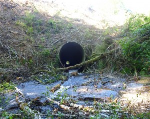
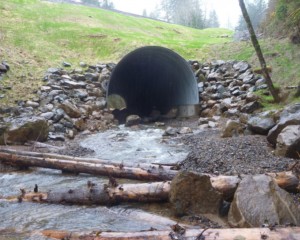
Figure 17. Undersized culvert with step blocked movement of Coho and Chinook to high quality upstream habitat (left). Culvert was removed and replaced with 26’ wide arched steel set onto concrete footings (right), allowing natural stream habitat to be maintained through the 126’ long passage. Source: CoosWA 2013

Riparian Cover Type

No applicable benchmarks to evaluate riparian cover type are currently in use in Oregon, but a diversity of conifer and deciduous trees, shrubs, and herbaceous cover is considered desirable. Conifers are particularly valuable, as their large size makes them well-suited to contribute LWD to stream channels and provide shade. Herbaceous cover (“grass”) alone is possibly the least preferred vegetative cover as it has limited potential to shade streams and its relatively shallow roots cannot hold soil together very effectively (CoosWA 2008). Riparian habitat parameters were assessed in CoosWA (2008, 2011c) and in Cornu et al. (2012).

As may be seen in Figure 19, grass is the predominant cover type throughout the evaluated drainage basins, with an average of 40% cover. In the subwatersheds’ lower reaches, this is likely due to agricultural and other human activities. The second most widespread cover type is shrubs, averaging 28% of cover throughout the evaluated areas. Deciduous tree cover averages 23% of the evaluated areas, and conifers, the least widespread of the cover types, average 6% cover. In some subwatersheds, such as Daniel’s Creek and Millicoma and lower South Fork Coos Rivers, average riparian conifer cover is only 2%.

In addition to evaluating riparian cover type, Robinson (2009) addressed the age of stands in the South Slough National Estuarine Research Reserve (a 6,000 acre natural area located in the Coos estuary and managed for long-term research, education, and coastal stewardship). They found that roughly 21% of the Reserve’s timber stands in the area were young (20-30 years old) and were regenerating from past harvests or other disturbances. By contrast, mature stands, defined as trees that are approximately 80-150 years old, comprise only about 3% of the Reserve. The majority of stands (76%) in the Reserve were between 40 and 80 years old in the competitive exclusion phase of forest development, meaning that these are high density stands dominated by similarly aged trees limiting the growth of understory vegetation.

The distribution of land use between forestry, agriculture, and rural residential uses (excluding the South Slough Reserve) is shown in Figure 20 and demonstrates how much of the watershed is managed for young forests, rather than the mature forests that would be more beneficial to riparian habitat. However, alternate uses of watershed area (agriculture, residential) may be even less amenable to vegetative cover, so the high percentage of the Coos watershed which is forested may actually represent an opportunity to improve riparian habitat more effectively than in other, more urbanized or agricultural watersheds.

Shade

The CoosWA’s 2006 assessment used photographs from 2002 U.S. Bureau of Land Management (BLM) aerial surveys to run a SHADOW model that estimated both potential and actual shading of subwatersheds on the north side of the Coos estuary. The model was used to examine three types of stream reach: upper stream reaches (steep gradient, forested narrow canyons), upper valleys (well-drained valleys with some elevation change), and lower valleys (poorly-drained, with very little elevation change). Shade data were collected in the field to check the model’s accuracy.

SHADOW model results indicated that while shade in the steep canyons of subwatersheds’ upper stream reaches was relatively close to reaching its potential, shade values dropped dramatically in both upper and lower valley areas. This likely reflects the contrasting vegetation cover associated with industrial forestry and agricultural land uses in local subwatersheds. Figures 21, 22 and 23 illustrate the disparity between potential and actual values of riparian shade in different reaches of the subwatersheds to which the SHADOW model was applied.

ODFW benchmarks for shade cover are for streams with an active channel width <12m, less than 60% shade cover is undesirable and more than 70% is desirable, and for streams >12m wide, less than 50% shade cover is undesirable and more than 60% is desirable (Foster et al. 2001).

The CoosWA and Cornu et al. assessments did not compare riparian shade analyses using ODFW benchmarks. Though we do not know the size of reaches from their shade analyses, ODFW’s benchmarks can still be generally applied. All of the upper reaches met both the <12m and >12m benchmarks for desirable shade cover. The upper valley reaches were more mixed; Willanch Creek failed to meet any benchmark while Daniel’s Creek, Echo Creek, and Kentuck Creek exceeded the most stringent benchmark (streams <12m (70%)). The reaches in the lower valleys were the least able to offer shade cover. Larson Creek and Echo Creek were the only streams to meet or exceed the minimum benchmark for streams >12m (50%). All other lower valley reaches failed to meet any benchmarks.

By reducing riparian shade on a stream, solar load is increased, raising stream temperatures, which in turn lowers dissolved oxygen (DO). There are 19 streams in the project area listed as water quality impaired for temperature and four water bodies are listed as water quality impaired for DO under USEPA’s Clean Water Act (section 303(d))(Figures 24 and 25). Many of these streams are considered limited for salmon rearing due to year-round high temperatures. DO is the oxygen available for aquatic fauna and is directly related to water temperature; slow moving, high temperature waters contain less DO than cool, fast flowing waters. Low dissolved oxygen levels affect resident fish, juvenile salmon rearing and aquatic life in general. For more information on temperatures and dissolved oxygen levels of water bodies in the project area, see the Physical Factors summary in Chapter 9: Water Quality.

Habitat Limiting Factors Model (HLFM)

The HLFM, used in some of the CoosWA assessments (2006, 2008), was designed to identify those habitat factors that limit Coho salmon populations and smolt production capacity in coastal Oregon watersheds (Nickelson 1998). In effect, the model identifies resource “bottlenecks,” which resource managers can address to help improve Coho salmon populations. The HLFM focuses on the amount of pool habitat in stream reaches, particularly beaver ponds and off-channel pool habitat. The model evaluates winter habitat capacity by total beaver and off-channel pool habitat, and summer habitat capacity by quantifying total pool habitat (which includes beaver, off-channel, and main channel pools)(ODF 2003).

The HLFM bottleneck illustrated in Figure 26 is a habitat limitation that occurs (A) during winter juvenile Coho salmon migration; and (B) during summertime juvenile Coho salmon migration. A manager facing scenario A might consider devoting resources to off-channel pools that give Coho salmon refuge from high stream flow events. Faced with scenario B, managers might place a higher priority on improving total pool area and on strategies for maintaining or improving cold water refugia in Coho streams.

Pools

Pools in streams provide important habitat for juvenile and adult fish; the deeper and more abundant the pools, the greater the benefits are to fish. Pools can provide fish with refuge from both high-flow events (hydrologic refugia), when water velocity could damage fish, and low-flow events (cold water refugia), when high water temperatures could prove harmful. Furthermore, pool depths can provide refuge to fish from surface predators (Foster et al. 2001). Pools can also act as sediment traps, allowing silt, sand, and fine organics to settle out of the water column and leaving downstream reaches free of these fine particles, which might otherwise clog valuable gravel beds that salmonids use for spawning (Swales and Levings 1989).

In British Columbia, Swales and Levings (1989) observed age 1+ Coho expressing a decided preference for pools as rearing habitat. They also found that the growth rates on Coho salmon in pools were greater than the growth rates of those in mainstem river reaches. In the project area, Weybright (2011) found that juvenile Coho that remained in pools during winter had a significantly higher survival rate than those that exhibited more mobile behavior. It’s likely that the pools provided juvenile fish with refuge from wintertime high-flow events, allowing calories that might otherwise have been expended fighting strong currents to be devoted to growth. Given that salmon are powerful and efficient swimmers compared to other species such as sturgeon or lamprey (Verhille et al. 2014; Lampman 2011), it’s possible that pools may prove to be even more important refuge for non-salmonid fish species.

During warm and dry summer months, residual pool depth may serve as essential habitat for fishes by providing concealment and the cooler water temperatures necessary for their health and survival (Foster et al. 2001). In the Oregon Coast Range, May and Lee (2004) found that limited residual pool habitat resulted in severe crowding of fish seeking refuge during summer low flows, and was associated with population decreases over the course of the summer. In streams subject to high temperatures and low summer flows (likely to exacerbated in the future by the local effects of climate change), deep pools are critical to the survival of temperature-sensitive species like salmon.

Large Woody Debris (LWD)order Lyrica online

LWD provides fish with cover in streams, helps create pools through hydraulic scouring of stream beds, and enhances the quality of pool habitat for fish. LWD in streams also provides the substrate for the growth of microorganisms, which are the foundation of stream and riparian zone food webs (Cornu et al. 2012).

This data summary describes LWD conditions in project area streams in terms of LWD “pieces”, “volume”, and “key pieces.” LWD pieces measures the frequency with which LWD is encountered in streams, and LWD volume measures amount of LWD present. Large volumes suggest a more persistent LWD presence and higher levels of habitat complexity while lower volumes suggest relatively diffuse and transient wood presence (as smaller wood is more likely to decompose relatively quickly or be moved downstream during high-flow events)(Foster et al. 2001).

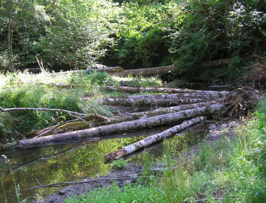
Figure 27. Tributary of the West Fork Millicoma River before (top right) and after (above) intentional placement of large wood pieces. Source: CoosWA 2009

Key LWD pieces, by contrast, are more likely to have an intense, sustained impact on stream ecology. Key LWD pieces are defined as those greater than 60 cm (24 in) in diameter and over 10 m (33 ft) long (OCSRI 1997). Larger LWD pieces are less likely to decompose quickly or to be moved during high-flow events. Key LWD pieces also anchor and retain other pieces of wood around which other material is deposited and trapped (Foster et al. 2001). Murphy and Koski (1989) found that key LWD pieces remained in streams significantly longer than smaller LWD, and their natural rates of replenishment was significantly slower than those of smaller pieces. Their research indicated that clear-cut timber harvesting without a streamside buffer could impair the ability of streams to replenish their stores of LWD for up to 250 years.

Alarmingly, a distinct lack of LWD was a defining feature of all evaluated subwatersheds of the project area. While certain individual reaches displayed adequate or occasionally even preferred levels of LWD, the overwhelming majority failed to meet even the minimum benchmark. This suggests that the introduction of LWD (especially key pieces) into stream habitats might be one of the most immediately effective ways to enhance stream habitat in the project area (Figure 27). Another way to encourage the future recruitment of LWD into project area streams is the management of riparian vegetation (see below) for the production of LWD. The simultaneous implementation of both strategies would generate immediate and long term benefits for project area streams and associated fish populations.

Gravel and Sediment in Riffles

Riffles are fast-water stream sections with surface turbulence, shallow, uniform cross-sections, gravel or cobble substrate and gradients of 1% to 4% (Foster et al. 2001). Riffles tend to occur more frequently in tributaries and higher mainstem stream reaches (CoosWA 2006). All salmonid species spawn in gravels associated with riffles, using the gravel to construct redds (depressions into which salmon eggs are deposited and fertilized)(Figure 28). Each salmon species prefers gravel of different sizes, allowing multiple species to reproduce in the same stream reach (Foster et al. 2001). It is therefore important that riffles contain sufficient amounts of gravel to support salmonid reproduction. Koski (1966) conducted studies in three Oregon streams which indicated that the composition of gravel within a redd was the single most important factor affecting the emergence of newly hatched Coho salmon.

Gravel in riffles is most useful when it coincides with low levels of fine sediments such as silt, sand, and fine organics (SSFO). Sediment is a natural component of stream beds, but excessive fine sediment can fill the space between gravel pieces, restricting oxygen flow to fish eggs and the macroinvertebrate communities which are the prey resources for juvenile fish. Koski (1966) also found that sedimentation negatively affected the survival of emerging salmon in Oregon streams, a phenomenon partially attributed to “entombment”, as newly hatched salmon starved to death while struggling to emerge from the stream bed.

Sedimentation of streams results from the chronic erosion of stream banks or other erodible watershed feature, or from sudden sediment depositions from episodic events such as landslides or culvert failures. A great deal of sedimentation, however, simply comes from unstable banks, often lacking vegetative cover and easily worn away by stream action.

Road-related Sediment and Bank Stability

Improperly designed or maintained roads and culverts are major sources of excess sediment loading in streams. Sedimentation can occur gradually, as road sediments are washed from road surfaces with traffic and heavy rain. Many factors contribute to sediment-filled runoff from roads, including road surface composition, distance between culverts or ditch reliefs, road slope, nearby forest and plant cover, road age, and road traffic volume (ODF 2003). This sedimentation can also be sudden and disastrous, as when a road fill slumps, a cut bank collapses, or a culvert washes out.

Even the best-constructed roads can pose a sediment hazard when located on high gradients near streams. In 2003, ODF released the Forest Practices Act, which included regulations on forest road construction (see sidebar)(ODF 2003c). ODF recommends maintaining existing roads as one of the best strategies for keeping road-related sediment out of watershed streams (ODF 2003).

A study conducted by CoosWA (2011b) found that ditch-relief culverts (structures designed to divert runoff from ditches to stable areas below roads) are very effective for reducing runoff and sediment delivery to streams. Many of the surveys discussed above recommended ditch-relief culverts.

Unstable banks contribute sediment to streams through collapse, slumping, chronic deterioration, landslides, and earth flows. Although a degree of erosion and occasional landslides occur naturally in healthy, dynamic stream systems, an excess of bank erosion or failure can lead to excessive sediment loading in streams.

The causes of bank instability can be natural or the result of human activity (particularly the clearing of streamside vegetation)(Figure 29). When riparian areas undergo human disturbances like development, agriculture, timber harvest, and fires, they often lack the plant cover necessary to stabilize stream banks. In fact, plant cover is so important to bank stabilization that 99% of uncovered banks in the Catching Slough and Daniels Creek assessments were considered unstable (CoosWA 2008). To become stable, a harvested riparian area must be replanted. In coastal Oregon, replanted stream banks will be considered stable after about 30 years of riparian vegetation regrowth (CoosWA 2008). According to USEPA, healthy watersheds cannot have more than more than 10% unstable (typically uncovered) banks; in some of our watersheds, unstable banks make up twice that percentage (USEPA 2012; CoosWA 2006, 2008, 2011c; Cornu et al. 2012).

Riparian Cover Type and Shade

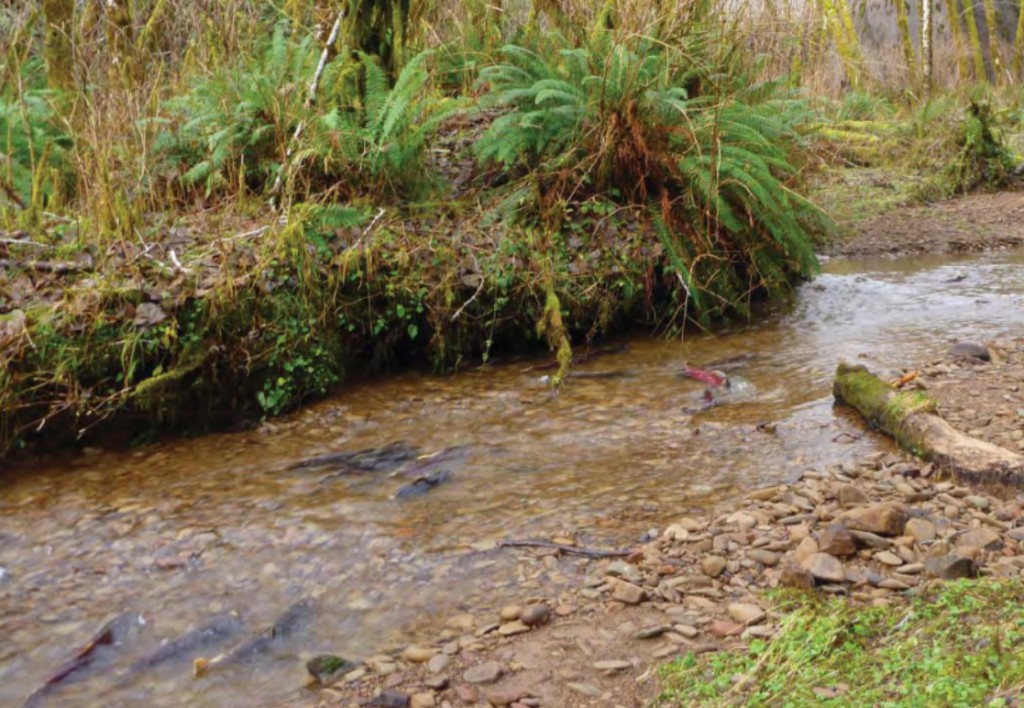
Figure 28. Coho building redds in gravel in a coastal Oregon stream. Source: CoosWA 2011a

Riparian vegetation provides a range of functions for steam habitat and water quality: it’s the major source of stream LWD, it helps keep stream banks stable (Foster et al. 2001), and it provides important nutrients and habitat for macroinvertebrates and other wildlife (Romero 2003). Vegetation shades streams and pools, moderating temperatures, especially during the summer (Foster et al. 2001).

The provision of stream shade is one of the most important functions provided by riparian vegetation, which plays a critical role in maintaining cold water refugia for salmonid and other fishes. Salmonids become stressed above 18˚ C (64˚ F), and the incipient lethal temperature for many salmonids occurs around 24˚ C (75˚ F). Particularly during the summer, intense sunlight combined with relatively low stream flows can make exposed stream reaches uninhabitable for fish. Shade keeps riparian habitats relatively cool and habitable (Foster et al. 2001).

Shrubs and trees in riparian zones provide food and dam building materials for beavers. Beaver activities provide pool complexes used as rearing habitat by juvenile salmonids which also function as sediment traps in stream systems.

Riparian vegetation also enriches local stream system food webs. Red alder (Alnus rubra), a common riparian zone tree in coastal Oregon, is notable for fixing nitrogen from the atmosphere which is then contributed to stream systems through extensive leaf litter and woody material (Compton et al. 2003). Large conifers, by contrast, provide the key LWD pieces that act as shelter for salmonids and create essential scour pool habitat (ODF 2003).

The relative scarcity of large conifers in reaches evaluated by CoosWA may be due in part to riparian vegetation clearing for residences and agriculture activities (particularly in the lower reaches), in addition to legacy timber harvests. In large portions of the project area, legacy forestry practices and current timber harvest rules determine the species composition and density of the riparian forests that border project area streams.

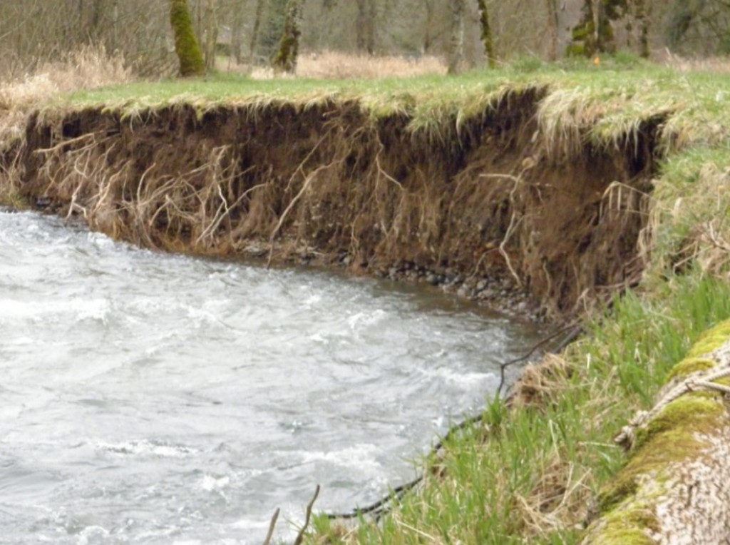
Figure 29. An eroding stream bank on the Oregon coast, which has been facilitated by the removal of stream bank vegetation. Source: Clackamas County Soil and Water Conservation District 2015