Geographic Features: The Coos estuary comprises a wide variety of intertidal mudflats, channels, and marshes; upland habitats are dominated by highly productive coniferous forests.
Meteorology: The project area experiences wet winters and dry summers. There is no apparent trend in local climate variability.
Hydrology: Ocean tides and freshwater from rivers and streams determine the quality and distribution of estuarine and riparian habitats.
Geology: Tectonic activity causes the incremental uplift of project area lands which historically have given way to sudden land subsidence during infrequent earthquakes.
Land Cover/Land Use: Land cover and land use have been mapped frequently since 1900, but different methods, resolution, focus and classifications make direct comparisons challenging.
Human Infrastructure: 76 miles of functioning dikes are protecting 17,300 acres of developed land in the project area; impervious surface area is increasing; road density exceeds thresholds for healthy watersheds.
This section includes the following data summaries: Geographic Features, Meteorology, Hydrology, Geology, Land Use/Land Cover, and Human Infrastructure — which describe physical properties of the Coos estuary and lower Coos watershed.
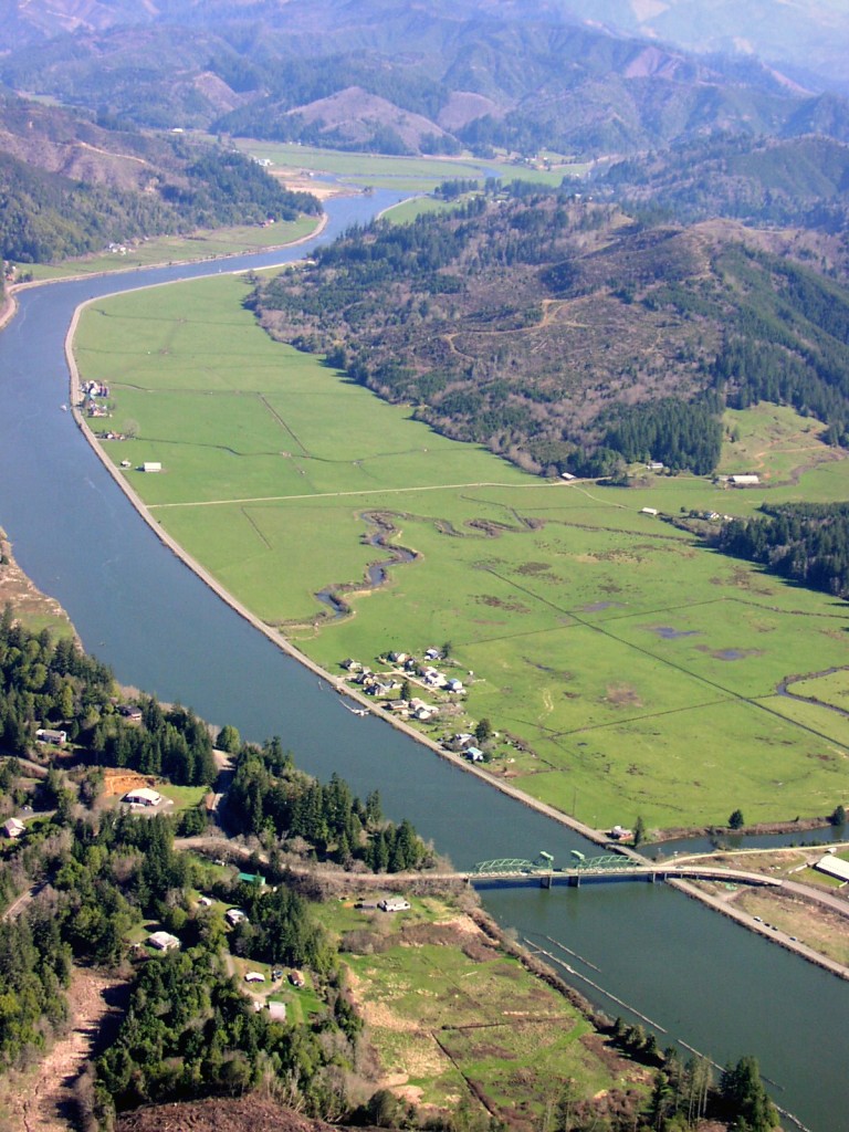
Coos River
It additionally describes different estuarine regions, and the watershed size for the major slough subsystems and tributaries. Changes to the project area lands from pre-contact conditions are discussed as well.
Much of the information supporting the Geographic Features data summary came from agency reports (e.g., Rumrill 2006, CoosWA 2006), peer-reviewed publications (e.g., Hickey and Banas 2003), and academic theses (e.g., Hyde 2007). Data used to create shoreline maps and describe the size of the Coos estuary and its subsystems were provided by the Oregon Ocean Coastal Management Program (OCMP), a project led by the Oregon Department of Land Conservation and Development (DLCD 2011).
Information from the OCMP Coos estuary data was compiled from multiple shoreline data sources. The majority of those data were derived from the National Oceanic and Atmospheric Administration’s (NOAA) Continually Updated Shoreline Product (CUSP). The CUSP shoreline was defined as the line of contact between land and water at approximately Mean High Water using Light Detection and Ranging (LiDAR) data or digital imagery interpretation.
Bathymetry information came from the United States Army Corps of Engineers (USACE 2014) hydrographic surveys, and surveys by Oregon State University scientists (Wood and Ruggiero 2014).
Information relating to ocean influences come from a variety of sources. The local sea level rise rate and tidal amplitude information were taken from NOAA’s Tides and Currents Charleston Station (NOAA 2015). Flushing times were informed by graduate thesis work from the mid-1970’s (Arneson 1976). Newly collected, unpublished data from the South Slough National Estuarine Research Reserve (SSNERR) were used to describe estuary currents (SSNERR 2015). Upwelling patterns for the Pacific Northwest came from the Northwest Fisheries Science Center website (NWFSC 2015).
Freshwater discharge data were compiled from existing reports (e.g., Cornu et al. 2012) and data from on-going stream monitoring efforts (USGS 2015b). Spatial information describing stream size and type was based on Oregon Department of Forestry Geographic Information System (GIS) streams data (ODF n.d.).
1. SSNERR’s System Wide Monitoring Program (SWMP) data. SWMP is a long term monitoring program that collects a variety of water quality and meteorological data. In this data summary, meteorological data from 2007-2014 were used, which included air temperature, precipitation, wind speed and direction, and photosynethically active radiation (PAR)(SWMP 2015).
2. North Bend Municipal Airport (Airport) meteorological data provided online by the Western Regional Climate Center (WRCC n.d., MesoWest 2015). We used air temperature, precipitation, and wind speed and direction data from 1931-
2014.
Since it is the largest available data set and represents the most complete record of long-term meteorological trends, we used the Airport data wherever possible. Additionally, because the Airport is closer to the geographic center of the project area, data from this monitoring station may be considered generally more representative of the project area as a whole. In cases where Airport data were not available (e.g., PAR), the SWMP data were used as alternatives.
In addition to the above-mentioned sources, the Meteorology data summary describes the Pacific Decadal Oscillation. This information is available through the Joint Institute for the Study of the Atmosphere and Ocean (JISAO 2015). Wind speed and direction data were analyzed and the associated figures were generated using Openair, a statistical package developed by Carslaw and Ropkins (2012).
Spatial data used to support the Geology data summary came from multiple sources. The Oregon Department of Geology and Mineral Industries (DOGAMI) compiled geological data for Oregon from various state and federal agencies, student theses, and consultants as part of a six year project (DOGAMI 2009). This data set enabled us to characterized the faults and folds within and near the project area. The United States Geological Survey (USGS 2005b) provided spatial information characterizing the locations of those faults and folds in the U.S. believed to be sources of significant earthquakes (those of magnitude 6 or greater) during the past 1.6 million years (paleoseismic earthquakes). These USGS data also provided information on age, direction and rate of slippage, angle and direction of dip, visibility, and type (e.g., strike-slip, normal, reverse, thrust) of each paleoseismic fault.
Landslide spatial information came from DOGAMI (2014) efforts to compile previously mapped landslides, LiDAR-based mapping of landslide features, and aerial photography review. It also included information on landslide classification, depth of failure, movement type, and confidence of interpretation (i.e. that the features called landslides are actually landslides), along with known costs associated with damage and losses. This dataset was cropped to the project area to identify landslide-prone areas where historic landslides have occurred.
Distribution of lands at high or moderate debris flow risk was provided by Oregon Department of Forestry (ODF 2000a). This dataset was derived from USGS Digital Elevation Models (DEMs) of the project area landscape; DEMs are used to evaluate slope steepness, stream channel confinement, and shape of debris flow deposits (fan shape). Historical information on debris flows was also used to inform the USGS dataset.
USGS (2015a) is a compilation of earthquake metrics (e.g., magnitude, amplitude, hypocenter, etc.) measured by contributing seismic networks, such as the Pacific Northwest Seismograph Network, the Oregon State University Geophysics Group, and the University of Oregon Department of Geology.
Two extensive, multi-year sources of recent LULC data were used for this summary: the National Land Cover Database (NLCD) and the Coastal Change Analysis Program (C-CAP).
The NLCD was developed by a group of U.S. federal agencies called the Multi-Resolution Land Characteristics Consortium (MRLC), and is based on Landsat satellite imagery and supplemental data sources (Homer et al. 2012). NLCD spatial data are available for the years 1992, 2001, 2006, and 2011. These data are national in scope and have 16 general land use and land cover classes, plus four vegetation types used for Alaska only. Only the classes relevant to the project area are included in the LULC data summary as outlined in its Table 1. The 1992, 2001, and 2006 editions of the NLCD data were retrofitted to enable comparisons with the 2011 dataset (Fry et al. 2009; Sohl, pers. comm, 2015).
The 2011 NLCD data are based primarily on a decision-tree classification of Landsat data (Homer et al. 2012).
Areas near the U.S. coastline are also included in the C-CAP land cover data from NOAA (C-CAP 2014). Land cover change for Oregon is available for the years 1996, 2001, 2006 and 2010. NOAA is one of the member agencies for the MRLC, so C-CAP land cover data are similar to NLCD data. Both are based on remotely sensed imagery, at 30 meter resolution, and both try to update their data sets every five years. The primary differences between the C-CAP and NLCD classification schemes are:
1. C-CAP distinguishes unconsolidated shore materials from other “barren” lands; and
2. C-CAP includes several additional wetland classes that NLCD does not.
However, both classification schemes can be aggregated to nine LULC categories: agriculture, barren (bare land), developed/urban, forest, grassland, scrub/shrub, water, emergent wetlands, and woody wetlands.
Additional data sources, a 1970’s USGS data set (USGS 2005a), Oregon Department of Forestry’s (ODF) ground surveys between 1895 and 1898 (ODF 2000b), and a Potential Natural Vegetation map developed from 1938 data by Tobalske and Osborne-Gowey (2002), provide “snapshots” of past LULC mapping efforts. However, because these maps differ in source materials, methods, resolution, and classification schemes, they cannot be directly compared to the recent NLCD or C-CAP data.
Finally, two models designed to project land cover patterns into the future are briefly described in the data summary. Models described are:
1.) Coastal Landscape Analysis and Modeling Study (Kline et al. 2003) ; and
2.) a GIS-based, deterministic model created by ODF (2014).
1) location and condition of, and management responsibility for levees;
2) location of tide gates;
3) location and percent cover of impervious surfaces;
4) location of stormwater outfalls; and
5) location and density of roads.
Most data were derived from analyses of existing spatial data (e.g., OCMP 2011a), but several reports were used to augment these data (e.g., NOAA 2010).
Thresholds for maximum recommended densities for impervious surfaces and roads referenced in the data summary came from a variety of sources, including agency reports (e.g., USEPA 2014) and peer-reviewed literature (e.g., Forman and Alexander 1998).
Spatial data describing project area levees and tidegates came from an OCMP geospatial database that uses LiDAR data and aerial photography (OCMP 2011a, b, c). The original purpose of this dataset was to provide coastal managers with quantitative information about levees and tide gates in Oregon estuaries. Location and condition of levees were digitized from LiDAR products and verified by field ground truthing and “participatory mapping,” where local experts in each estuarine system were asked to offer their best professional judgments.
Information about levee-protected lands was derived from tax-assessor maps, by identifying tax parcels immediately adjacent or abutting levees (OCMP 2011b).
Tide gate locations were identified from local inventories (e.g., ODOT tide gate locations, fish passage barriers, restoration projects), local expert knowledge, and on-the-ground investigations, then digitized with the benefit
of LiDAR landscape contour and elevation data (OCMP 2011c).
The impervious surface data are products of the NLCD provided by MRLC, created for the years 2001, 2006, and 2011 (MRLC 2015).
MRLC’s Percent Developed Imperviousness maps were created by:
1) classifying images with a nominal spatial resolution of 1 meter into pervious or impervious surfaces and summed within 30-meter Landsat pixels to obtain a percentage;
2) using the reference data and Landsat spectral bands to calibrate density prediction models; and
3) spatially extrapolating the models for per-pixel imperviousness (NLCD 2001 metadata).
Stormwater outfall locations were provided by the Cities of North Bend and Coos Bay for outfalls within their city limits (City of North Bend 2005, City of Coos Bay n.d.). Roads spatial data came from the Oregon Department of Transportation’s statewide compilation of roads (ODOT 2014).
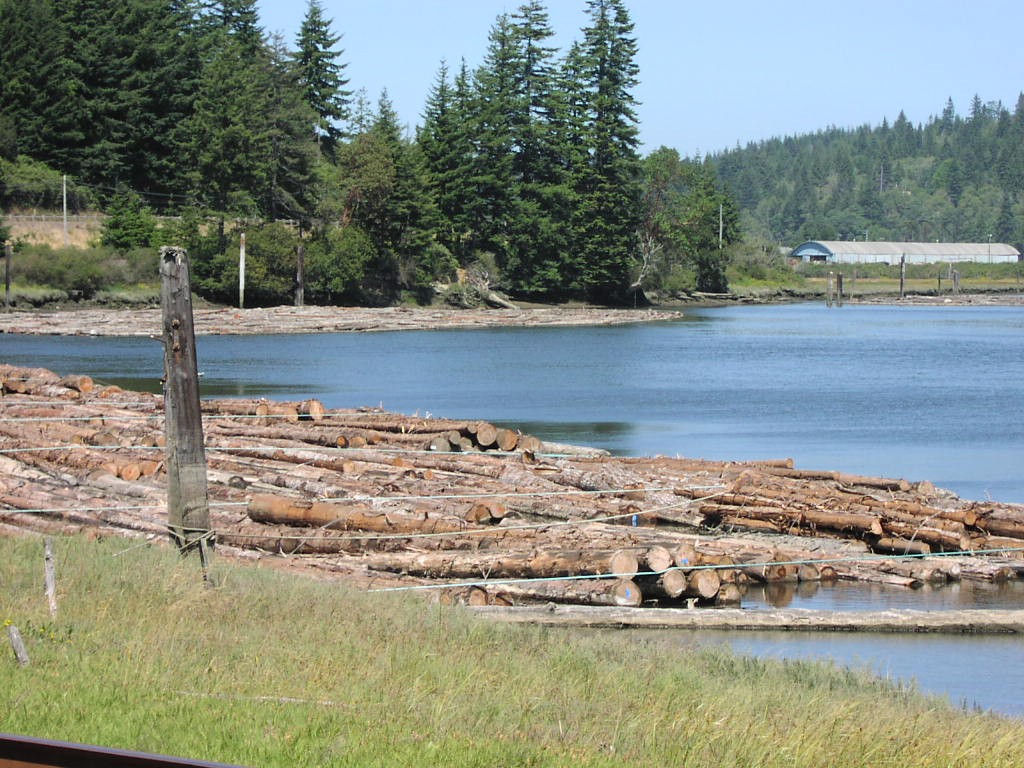
Isthmus Slough log raft
The National Oceanic and Atmospheric Administration (NOAA) Coastal Services Center created maps to show predicted sea level rise inundation extents ranging from 1-6 ft (above MHHW)(USDOC 2012).
These maps inform coastal managers and scientists about related coastal flooding impacts. Scenarios were created using a modified bathtub model, which accounts for local/regional tidal variability and hydrologic connectivity. Data used to create the model came from DEMs and a tidal surface model (which was created with NOAA’s VDatum in conjunction with spatial interpolation/extrapolation methods). Models do not take into account potential erosion scenarios.
Data Gaps and Limitations
Geographic Features: Some of the information presented in the Geographic Features data summary may be dated, because the best available information came from an Oregon Department of Fish and Wildlife report from 1979 (Roye 1979).
Hydrology: Our understanding of tidal hydrology in the Coos estuary is limited or dated information. Bathymetry data (bottom contours) are available for the main shipping channel in the Coos estuary but elsewhere the data are severely limited. The incomplete nature of bathymetry data affects our ability to more fully understand tidal flushing rates in the estuary because these rates are largely based on estuarine bathymetry. In addition, the tidal flushing rates reported in the data summary are referenced from a 1976 report (Arneson 1976) which will not reflect changes which have taken place in the estuary since then (e.g., changes in the size of the Coos estuary’s commercial shipping channel).
Head of tide information came from a 1989 Oregon Department of State Land (ODSL) report, which was then digitized into a GIS shapefile using both on-screen and manual digitization methods in 2000 (ODSL 2000). The methods detailing how head of tide locations were determined in the 1989 report were not included in the original publication and the authors are since deceased. Heads of tide locations appear to include major tributaries only; minor tributaries were excluded. Many heads of tide locations for the project area include observation dates, but not all.
Years of listed observations were in different years (either 1979 or 1984) and months (March-July). Observations were all made during high tides, but whether or not they were made during the highest high tide of the day was not mentioned (it’s a logical to assume they were but this is not confirmed in the source material). Likewise, it is unknown if high river and stream flows were accounted for.
Meteorology: The Meteorology data summary makes use of two meteorological monitoring stations in the project area:
1) the North Bend Municipal Airport monitoring station (WRCC n.d., MesoWest 2015); and
2) SSNERR’s meteorological monitoring station located in Charleston (SWMP 2015).
Two additional stations are located in the project area (NOAA’s Climate Reference Network station in upper South Slough and the meteorological monitoring station associated with the NOAA tide station in Charleston), but were not used
because these data sets are not as complete as the Airport and SWMP data. Furthermore, the locations of the unused data are encompassed by the Airport and SWMP sets.
The analysis of project area meteorology data was limited by the resources available. The two stations we used oftentimes produced vast data sets (some data collected multiple times per hour for the past 10-20 years), comprehensive
analysis of which was beyond the scope of this project. While we were able to use those data to characterize basic meteorological status and trends for the project area, we feel there would be significant benefit to making a special effort to secure funding to complete a more robust analysis of those large data sets.
The meteorological data are subject to quality assurance and quality control (QA/QC) concerns (e.g., equipment malfunction, instrument recording error, failure to deploy instrument, instrument calibration issues, etc.). Data that have been compromised by QA/QC concerns were dropped prior to analyses. In rare cases, the validity of wind speed data from the MesoWest (2015) dataset were called into question even in the absence of any QA/QC flags.
Observations from these data meeting the following illogical or unlikely conditions were removed prior to analysis:
• Sustained wind speed exceeds the speed of wind gusts.
• Unlikely high sustained wind speed (e.g., 129 mph reported on July 12, 2005)
• Unreasonably large gap between sustained wind speed and speed of wind gusts (e.g., sustained winds of 6 mph and wind gusts of 92 mph reported on October 25, 2012)
It is important to note that the removal of questionable observations from these data sets does not obscure seasonal or long-term trends, because the number of compromised data points represents a very small percentage of all meteorological observations. We also favored the use of the SWMP (2015) data for precipitation analyses since the MesoWest (2015) data included several thousand observations indicating the highly unlikely occurrence of storm events during which the amount of local precipitation received in a 24-hour period met or exceeded 60 inches (the approximate annual precipitation total for the project area).
SSNERR staff maintain the SWMP meteorological monitoring station. From 2007-2014 this station was located on the University of Oregon Institute of Marine Biology (OIMB) campus in Charleston near the northern end of the South Slough Subsystem. In December 2014, OIMB installed a new wind turbine in proximity to the SWMP monitoring station which raised concerns about the turbine’s potential effects on the station’s data. As a result SSNERR is relocating the SWMP meteorological monitoring station.
Beginning in 2016, data collection will occur at a new location in Tom’s Creek Marsh near the southern end of the South Slough Subsystem. Although this data summary reports only data occurring prior to 2016 (i.e., prior to the move),
it should be noted that future comparisons of pre-2016 meteorological SWMP data to post-2016 data should be made with caution because of this change.
This data summary uses a technique called “time series decomposition” to examine the data for long-term air temperature and precipitation trends. Although this method shows that no trends are immediately apparent for air temperature or precipitation in the 80-year data set, it should be noted that this does rule out possible longer-term trends for the project area. For example, it’s feasible that an overall warming trend in the project area may have occurred since the Industrial Revolution (early 18th century). However, since data are only available starting in the early 20th century, it could be the case that this warming trend is not detectable because the time horizon of the available data may be too small to detect any true long term trend.
Analyses of changes in the frequency and intensity of storm events requires access to very high resolution data over a very long time period. To understand the intensity of a storm, one must have access to complete and highly detailed meteorological records (e.g., precipitation received per hour). Although the SWMP (2015) dataset provides precipitation data at this level of detail, it includes only seven years of data (2007-2014), which is not enough time to facilitate meaningful analyses of change in storm frequency and intensity. Furthermore, the 80-year MicroWest (2015) data set only provides precipitation totals over 24-hour periods, subject to the QA/QC concerns mentioned above. At this point, the currently available meteorology data do not appear to lend themselves to support meaningful analyses of changes to storm frequency and intensity in the project area. For the reasons listed above, we suggest that additional data collection and analysis is needed to fully understand meteorology trends in the project area.
Geology: Several caveats should be noted about the spatial data sets used in the Geology data summary. First, it’s likely that the DOGAMI (2014) landslide data are not comprehensive for the project area; not all landslides were identified in the data. This information is a compilation of several data sources which varied in scale and accuracy. Second, debris flow spatial data provided by ODF (2000) should be used for general information, and not used to determine actual hazards at any given location. Hazard values were based on slope, basin area, and rock formation. On-the-ground verification was completed to check mapping accuracy. Horizontal accuracy at the 1:24,000 scale was about 45 ft. Third, the accuracy of the fault and fold information from DOGAMI (2009) may be limited because it’s a compilation from various data sources; accuracy varies according to the source data.
However, it should be noted that in the process of creating this dataset, DOGAMI did check for discrepancies between sources and made adjustments as needed. Finally, fault and fold data from USGS (2005) is intended to be used at 1:250,000 or smaller scales, which is smaller scale (i.e., bigger area) than the project area. The accuracy at their intended scale equates to 450 ft for fault/fold line placement.
Land Use/Land Cover (LULC): Data accuracy varies by geographic region and specific LULC classes. The data are most accurate when applied to regional or national analyses, rather than local evaluations. The accuracy of these data for our study area is unknown and would require local information and additional analysis to determine.
Overall accuracy in the Pacific Northwest was determined to be 83% (standard error = 2%) for NLCD 1992 Anderson Level I classes, and 63% (standard error = 2%) for Level II (Wickham et al. 2004). Level I classes comprise broad categories; Level II classes comprise more specific categories. A comparison of NLCD 1992 with similar data in Rhode Island and Massachusetts revealed acceptable accuracy for developed land, agriculture, forest,and water, but consistently poor classifications for rangeland, wetlands, and barren lands (Hollister et al. 2004). In the 2001 NLCD data, the region encompassing coastal Oregon had an overall “user’s accuracy” of 79% at Level II, but varied from 20% for woody wetlands to 98% for high-intensity developed land (Wickham et al. 2010). The “user’s accuracy” measures the probability that the mapped classification corresponds to what is on the ground (Congalton 2005). Wickham et al. (2010) reported a substantial improvement in the national accuracy of forest and cropland classes from the 1992 data to the 2001 and 2006 data. On the other hand, the user accuracy for land cover change between 2001 and 2006 for the same region was below 50% for the classes agriculture gain, agriculture loss, water loss, and forest gain (Wickham et al. 2013). All NLCD data are considered “provisional” until a formal accuracy assessment is done and is not yet available for the 2011 NLCD.
In addition, unlike previous years’ NLCD classifications, the 2011 NLCD data for the Coos Bay area excludes the estuary itself- the water body. This important data gap confounds direct comparisons among years based on subsystem land cover percentages. To compensate for this discrepancy, percentages for NLCD 2011 data were calculated using the land areas without the estuary and also by approximating the estuary extent by inserting the 2006 NLCD data. Another land cover class affected by the depiction of the estuary is the “Barren” or “bare land” category because mudflats and other shoreline areas may or may not be visible in the satellite imagery. Apparently the images show low tide in some
years and high tide in others, thus the water and Barren percentages fluctuate.
Because C-CAP and NLCD are based on the same source information, it’s assumed that overall accuracy for the shared land cover types are generally the same. In the C-CAP data, small areas classified as perennial ice or snow were assumed to be errors caused by bright reflective surfaces including, but not limited to, temporary frost, snow, or ice. Because the snow/ice errors were less than 0.1% of the study area, the data were retained “as is”.
Neither the NLCD nor the C-CAP data distinguish between natural forest and trees managed for timber production. It is important to recognize several differences between the 1970’s data (USGS 2005a) and subsequent land cover maps. First, different methods, source materials, and classification schemes were used. Second, the 1970’s maps were also substantially coarser (larger minimum mapping unit) than subsequent data, with an unknown accuracy rate. The 1970’s
data, and other historic data, are presented in the data summary to indicate general land cover trends and the evolution of LULC data over time.
The ODF (2000b) map depicting timber production and burned areas in the project area is also less detailed due to its small scale (1:500,000). It does not include all land cover categories, therefore cannot be used for direct comparisons with more recent classifications. Similar issues regarding spatial and categorical resolution also exist for the pre-settlement vegetation map (Tobalske and Osborne-Gowey 2002).
Human Infrastructure: The coarse-scale OCMP data, which were used to highlight lands in the project area excluded from tidal flooding (currently or historically) by levees (Figure 5 in the Human Infrastructure data summary), are derived solely from tax assessor data. No hydrology or elevation data were used to estimate tidally-excluded acreage. Therefore, some lands not meeting the simple mapping criteria would be excluded from the map (e.g., low lying parcels not adjacent to a levee, or uplands adjacent to levees). OCMP (2011c) tide gate information is very useful but appears to not be a fully comprehensive inventory since it was largely based on existing information and without the benefit of additional systematic field surveys. According to the metadata associated with the NLCD 2010 Percent Developed Imperviousness data, the accuracy of zone 2, which encompasses the study area, is 86.7%.
A study by Roy and Shuster (2009) found that field measurements of Total Impervious Area (TIA) were considerably higher than the NLCD values in a small suburban basin in Cincinnati, Ohio. Use of the NLCD-based data in this study may therefore under-estimate the actual percentages of impervious surfaces for the project area. Roy and Shuster also recommend on-site assessments to accurately map Directly Connected Impervious Areas (DCIA): those impervious surfaces that drain storm water directly to specific waterways through storm drains. Neither DCIAs nor semi-impervious areas (such as compacted soil) are described in this data summary because no reliable data are currently available. Although
some coefficients have been developed for estimating DCIA as a function of land use in the Northeastern United States (USEPA 2014), these values have not been evaluated for use in the project area.
Storm drain outfall locations were only available for the cities of North Bend and Coos Bay. Spatial information for outfalls in the project area are thus under-representative. ODOT (2014) spatial road data were compiled from numerous sources throughout the state, based on best available data from each road authority. We used data relevant to the project area. Data have been compiled and digitized differently by each jurisdiction and thus are subject to different levels of accuracy. ODOT does validate some of its data (e.g.,flags milepoints that are not logical). They assume a 1:24,000 accuracy for the entire state. The data used in this summary are ODOT’s public data and do not include roads whose locations were restricted for distribution.